8 Adaptive basis functions
We can avoid using kernels, and try to learn \phi(x) directly from data. That is, we will create an adaptive basis function model of the form f(x) = w_0 + \sum_{m = 1}^M w_m \phi_m(x; v_m)
where \phi_m(x; v_m) is the m-th basis function, and v_m are the parameters of the basis function itself learned from data.
8.1 Bagging
8.1.1 Random forest
Let’s start considering decision trees. Recall that a decision tree partitions a space into regions, so we can associate a mean response to each of these regions. We can therefore write a decision tree in the following form:
f(x) = \sum_{m = 1}^M w_m \phi(x; v_m)
where w_m is the mean response in the region, v_m encodes the choice of variable to split on, and the threshold value, on the path from the root to the m-th leaf.
Decision trees are good because they can easily handle both discrete and continuous inputs, they perform automatic variable selection, they scale well to large datasets, and can handle missing inputs. The problem is that they are unstable: small changes to the input data can have large effects on the structure of the tree, due to the hierarchical nature of the tree-growing process. We say that trees are high-variance estimators.
A way to reduce the variance is using a bagging technique called random forest: we train M different trees on different subsets of the data as well as a randomly chosen subset of data f(x) = \sum_{m = 1}^M \dfrac{1}{M} f_m(x)
8.1.1.1 Extremely Randomized Trees
- Each tree is trained on the whole dataset
- Instead of computing the locally optimal split for each feature under consideration, a random split is selected
8.2 Boosting
Boosting is a powerful technique for combining multiple base learners (or weak learners) to produce a sort of committee. The idea is to train M base classifiers in sequence, and each base classifier is trained using a weighted form of the dataset: points that are misclassified by one of the base classifiers are given greater weight when used to train the next classifier in the sequence. Once all the classifiers have been trained, their predictions are then combined through a weighted majority voting scheme.
Now we see how AdaBoost works. Consider a two-class classification problem, in which the training data comprises input vectors x_1, . . . , x_N with corresponding binary target variables t_1, . . . , t_N, where t_n \in \{-1, 1\}. Each data point is given a weight w_n, initially set \frac{1}{N} for all data points.
AdaBoost
Initialize the data weighting coefficients \{w_n\} by setting w_n^{(1)} = \frac{1}{N} for n = 1, …, N
For m = 1, …, M:
- Fit a classifier y_m(x) to the training data by minimizing the weighted error function J_m =\sum_{n=1}^N w_n^{(m)} I(y_m(x_n) \neq t_n) where I(y_m(x_n) \neq t_n) is the indicator function and equals 1 when the model misclassifies, 0 otherwise.
Evaluate the quantities \epsilon_m = \dfrac{\sum^N_{n=1} w^{(m)}_n I(y_m(x_n) \neq t_n)}{\sum^N_{n=1} w^{(m)}_n} and then use these to evaluate \alpha_m = ln \left[ \dfrac{1 - \epsilon_m}{\epsilon_m} \right]
Update the weights. In this way, if an example is classified correctly, the weight is unchanged, while if it is misclassified the weight increases. w^{(m+1)}_n = w^{(m)}_n \exp\{\alpha _m I(y_m(x_n) \neq t_n)\}
Make predictions using the final model, which is given by Y_M(x) = sign \left( \sum^M_{m=1} \alpha_m y_m(x) \right)
\epsilon_m represents a weighted measure of the error rate of each base classifier on the dataset, while \alpha_m is the weight assigned to each base classifier.
Why \alpha_m = ln \left[ \frac{1 - \epsilon_m}{\epsilon_m} \right]? This is mathematically speaking the inverse function of the sigmoid function: the sigmoid function squashes values from (-\infty, +\infty) to (0, 1), in this way we are doing the contrary, we take the error rate in a probability form (because it is normalized by the sum of the weights) and we encode it outside the (0, 1) range.
8.2.1 Gradient Boosting
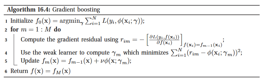
Gradient Boosting frames the problem as an optimization task. It treats the model building process as a form of gradient descent, but instead of descending in a parameter space, it descends in a function space. Each new weak learner is trained to approximate the negative gradient of a chosen loss function, which points in the direction that best reduces the overall error.
1. Initialize f_0(\mathbf{x}) = \text{argmin}_{\gamma} \sum_{i=1}^{N} L(y_i, \phi(\mathbf{x}_i; \gamma))
- This step creates the initial, very simple model, f_0(\mathbf{x}).
- L(y_i, f(\mathbf{x}_i)) is the loss function.
- \phi(\mathbf{x}; \gamma) represents a single weak learner with parameters \gamma
2. Compute the gradient r_{im} = -\left[\frac{\partial L(y_i, f(\mathbf{x}_i))}{\partial f(\mathbf{x}_i)}\right]_{f(\mathbf{x}_i)=f_{m-1}(\mathbf{x}_i)}
- For each data point i, it calculates the gradient of the loss function with respect to the model’s prediction from the previous step, f_{m-1}(\mathbf{x}_i).
- The result, r_{im}, is called a pseudo-residual.
3. Fit a weak learner to the residuals \gamma_m which minimizes \sum_{i=1}^{N} (r_{im} - \phi(\mathbf{x}_i; \gamma_m))^2
- The residuals r_{im} tell us the ideal direction to update our predictions. This new learner, \phi(\mathbf{x}; \gamma_m), learns the pattern of the previous model’s errors.
4. Update the Ensemble Model: f_m(\mathbf{x}) = f_{m-1}(\mathbf{x}) + \nu \phi(\mathbf{x}; \gamma_m)
- f_{m-1}(\mathbf{x}) is our ensemble model from the last iteration.
- \phi(\mathbf{x}; \gamma_m) is the new learner trained on the residuals.
- \nu is the learning rate
8.3 Stacking
Stacking combines the predictions of multiple base models by training a meta-model to make the final prediction.
1. Training the Base Models
- The training dataset is partitioned into K folds.
- For each of the K folds:
- A set of diverse base models is trained on the other K-1 folds.
- Each trained base model then makes predictions on the held-out fold.
- These “out-of-fold” predictions are collected. At the end of this process, we have a full set of predictions from each base model for every data point in the original training set.
2. Training the Meta-Model
- A new training dataset is constructed where:
- The features are the out-of-fold predictions generated by the base models.
- The target is the true label from the training data.
- The meta-model is trained on this new dataset. This model learns the mapping from base model predictions to the final correct outcome.
3. Prediction
To make a prediction on a new data point:
- The data point is first passed to all the base models (which have been retrained on the entire original training set for optimal performance).
- The predictions from these base models are collected and used as input features for the trained meta-model.
- The meta-model produces the final prediction.
In summary, stacking creates a hierarchical model structure where a meta-learner is trained to aggregate the intelligence of the underlying base learners, leveraging their diverse perspectives to improve overall generalization performance.